Cellular automata in science
A cellular automaton is a grid of cells, each holding a small state, updated all at once by the same rule applied to every cell and its neighbours.
Stanislaw Ulam and John von Neumann came up with the idea at Los Alamos in the 1940s: Ulam was studying crystal growth on a lattice, and von Neumann used a grid of cells to build a machine that could copy itself. One of the best-known examples is John Conway’s Game of Life, which Martin Gardner described in Scientific American in October 1970. In my llm-life demo, a small language model plays Life in your browser, one cell at a time. This post is about another use of the idea, as a way of doing physics, with the same kind of rule on a different grid.
Try the demo: flow
Read the code: github.com/ilnmtlbnm/jacobi2000
A gas made of bits
In 1973 Jean Hardy, Yves Pomeau and Olivier de Pazzis proposed a fluid made of particles on a square grid (J. Math. Phys. 14, 1746). Each particle moves along a link at every tick, and when two meet head on they leave at right angles. But on a square grid the gas does not flow like a real fluid: it favours the directions of the grid, and a flow at an angle to them comes out wrong.
Put an obstacle in a stream of fluid and it sheds a street of vortices behind it, turning one way and then the other. A famous and impressive example is wind blowing clouds past an island, where the vortices can be seen from space.
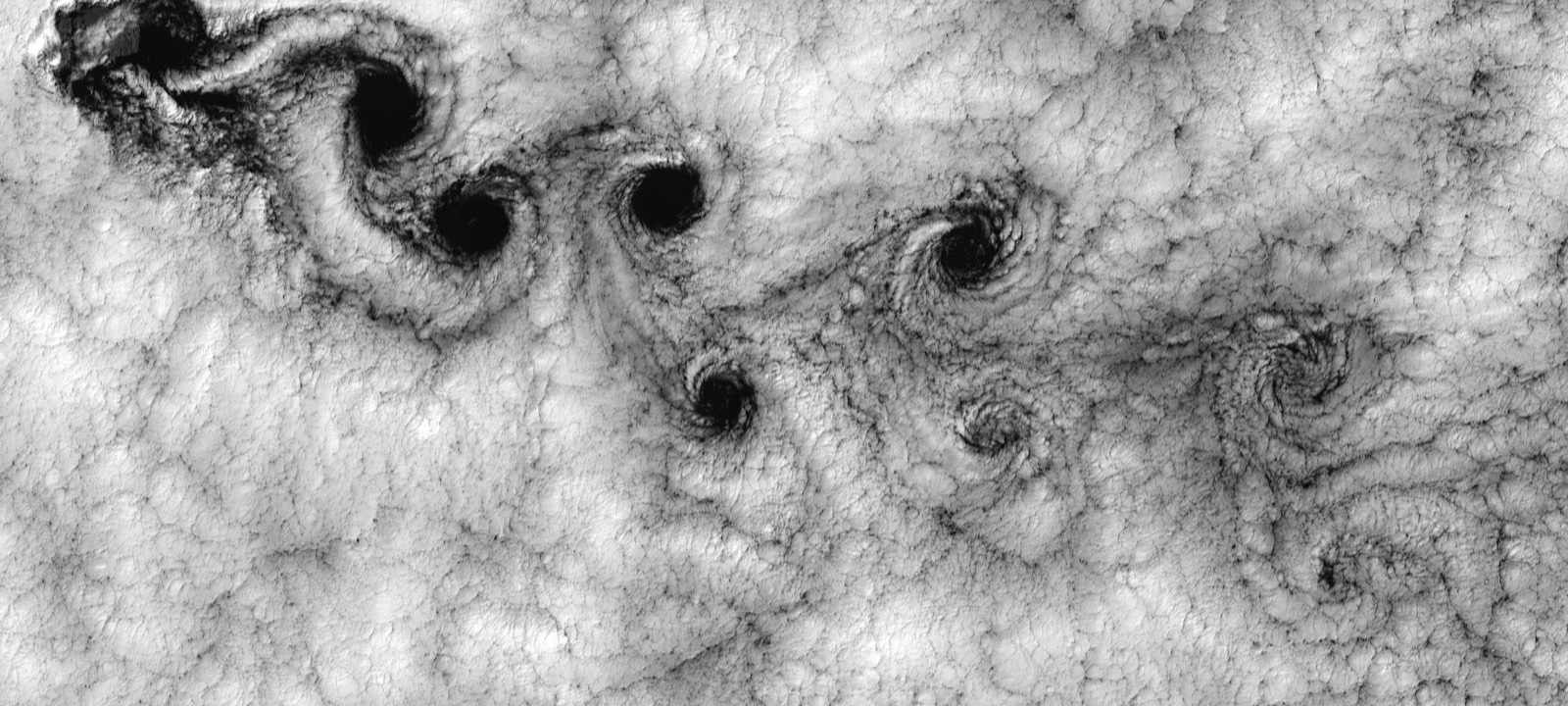
A von Kármán vortex street in the clouds downwind of one of the Juan Fernández Islands, off Chile, seen by Landsat 7 on 15 September 1999. The island is at the top left. Image: Robert Cahalan, NASA/GSFC, public domain, via Wikimedia Commons.

A lattice gas reproduces these vortices from a few simple rules. Its particles move along the six directions of a triangular grid, one step per tick, and collide at the nodes by a fixed rule. Nothing else is programmed: the flow around an obstacle and the vortex street behind it come from those collisions alone. In 1986 Uriel Frisch, Brosl Hasslacher and Yves Pomeau showed that on a triangular grid, where each node has six neighbours, such a gas of on-or-off particles does follow, at large scales, the Navier–Stokes equation, and that it can be used to design simple, massively parallel computing machines (Phys. Rev. Lett. 56, 1505). Their model is known as FHP, for Frisch, Hasslacher and Pomeau.
Here is one node of that grid and its six links, with the collision rule at its simplest.
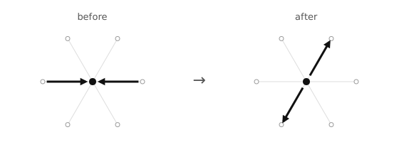
A node and its six links. Each link holds a particle or does not. Here a head-on pair collides and leaves rotated by 60 degrees (the rotation can go either way). The count of particles and the total momentum are the same before and after.
The Connection Machine
Danny Hillis’s Thinking Machines built the Connection Machine in the 1980s: a computer of about 64,000 very small processors that all run the same instruction at once. It is a perfect machine for cellular automata, because each processor can take one cell. A node of a lattice gas holds a few bits and follows the same rule as its neighbours.
In Richard Feynman and the Connection Machine, Hillis tells how Feynman first called the idea of a parallel computer with a million processors “positively the dopiest idea I ever heard”, then agreed to spend a summer at the company. The first program run on the machine, in April 1985, was Conway’s Life. Later Stephen Wolfram ran a lattice gas of the Frisch, Hasslacher and Pomeau kind on it and made a movie of turbulent flow in two dimensions.
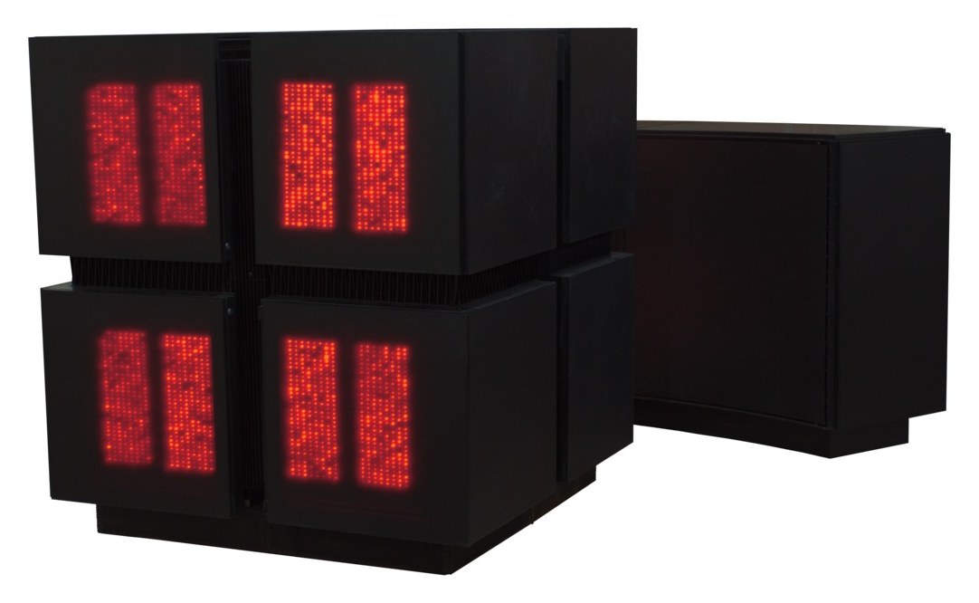
A Connection Machine CM-2 and its DataVault storage unit. Photo: Logg Tandy, CC BY-SA 4.0, via Wikimedia Commons.

The machine was then used for real fluid work. Bruce Boghosian, Washington Taylor, Daniel Rothman and Ralph Santos ran a two-colour variant of the triangular-lattice gas on a CM-2, at about 100 million site updates per second (talk slides). At MIT, the Information Mechanics group built a machine of its own for this kind of simulation, CAM-8, and its 1994 brochure shows a lattice gas flow in a channel.
In a browser tab
The flow page sets up the classic experiment: a channel, a flat plate across it, and fluid entering from the left at constant speed. Nothing else is imposed. After a couple of minutes the wake behind the plate becomes unstable and starts shedding vortices, first on one side and then on the other, at a Reynolds number of about 140.
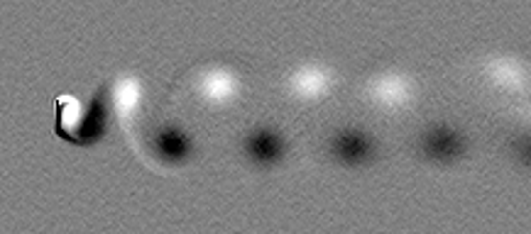
The page after a couple of minutes. The picture shows how the fluid spins. Black and white are the two directions of rotation on a grey background, and the further from grey, the faster it spins. The plate is at the left, the flow comes from the left, and the spots are the vortices it sheds.
The model is my own variant of FHP, which I call signed ternary. In FHP, each link holds one bit: a particle or no particle. In signed ternary, each link holds one of three values, −1, 0 or +1, measured against a reference.
The reference is the average flow, computed over blocks of 8 by 8 nodes: how many particles each of the six links should carry on average, given the density and the velocity of the fluid in that block. A link then only records whether it carries one particle more than that average, one less, or the same.
The smooth part of the flow is held by the references, and the links only carry the fluctuations around it. There is less noise, so the gas reaches a higher Reynolds number on the same grid.
As in the original FHP, each step has two phases:
- streaming: each value moves along its link to the neighbouring node;
- collision: each node looks up its six values in a collision table, and the nodes of the plate send every particle back where it came from.
Everything is computed in integers: mass and momentum are conserved exactly, and the GPU and the CPU give the same result bit for bit. I found no earlier lattice gas built this way. The full model, the averaging and the code are described in the technical report.
In pseudo code (the real code is in the source):
for every node x:
    for each of the six links d:
        v = value of link d at the neighbour it comes from
        shift = reference[neighbour][d] - reference[x][d]
        v = v + random_round(shift)
        v = clamp(v, -1, +1)
        link[d] = v
    if x is part of the plate:
        send every particle back where it came from
    else:
        new state = collision_table[link values, random bit]
A single node is still noisy, so the picture is averaged before it is drawn: it shows the spin of the fluid over blocks of nodes, averaged over time. The grid has about 1.6 million nodes (fewer on a phone).
The simulation is written in Rust and compiled to WebAssembly, following the design of my lean inference engine: one source for the GPU and the CPU, with the same results on both. It runs in a web worker, apart from the page, on the GPU through WebGPU when the browser has it, and otherwise on the processor’s threads. The worker runs the simulation and keeps the averaged field up to date; the page only asks for the latest values and draws them.
The CM-2 runs above reached about 100 million site updates per second, on a machine of 64,000 processors, nearly forty years ago. The flow page does about a billion, in a browser tab on a laptop.